This time, I want to share some Google Sheets formulas which work like magic. Let’s dive in!

Scenario:

There will be a monthly ingestion every start of the following month to the ‘raw’ sheet in the Excel file and the objective is to have a financial summary sheet that serves as an end-of-month report that updates automatically. So, on 1 January 2022, data for the month of December 2021 will be automatically ingested, hence we need an automated GSheet report to avoid manual labor at the start of every month.

Raw Sheet:

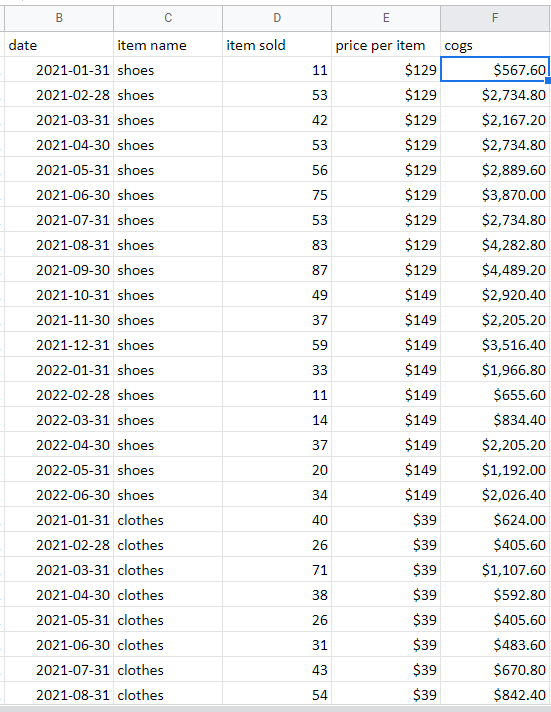
Raw Sheet by Author

Here’s an example of simple raw data containing the date, item name, item sold, price per item, and COGS.

1. ARRAYFORMULA

First, we want to add a Revenue column, Item Sold * Price per Item, next to the existing data; however, if we use the simple =D2 * E2 formula, we will have to update the sheet every time there are new rows of data.

To automate, we can hit Ctrl+Shift+Enter while editing a formula in the first row and use the ARRAYFORMULA function. Do not forget to add : Column in the end to make it an array formula instead of a single cell formula (for example, D2:D instead of D2) and it will automatically populate the below cells in the column with the formula result.

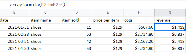
Example of Arrayformula by Author

However, do note that it will literally populate every cell of the column with the formula, which can leave unwanted results like 0 below:

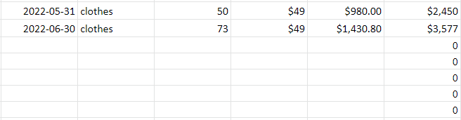
Illustration of Arrayformula error by Author

To avoid this, we can add an IF condition like so:

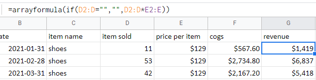
Example of modified Arrayformula by Author

Arrayformulas work wonderfully with a huge range of functions, such as SUMIFS(), YEAR(), IF(), etc. so do explore them!

In this case, we’ll also add the Year and Gross Profit column.

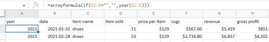
Example of Arrayformula with Year function by Author

2. MAX & EOMONTH

Once we get the raw data done, it’s time to design what the summary report will look like. For simplicity, we’ll use this design below which reports all the metrics by item name, month, and year.

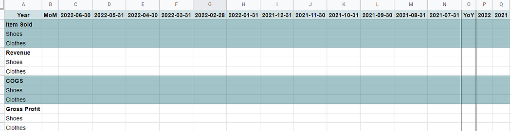
Summary report design by Author

Secondly, we want the months displayed in row 1 to be updated. To do that, we can use the MAX() function to get the most recent date from the raw data.

For the other columns, we can use the EOMONTH() formula because we want the last date of every month which falls one of month before, hence -1, the date on its left.

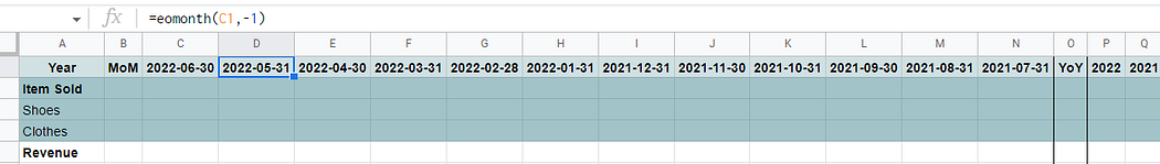
Example of EOMONTH function by Author

3. SUMIFS

Next, to fill the report, SUMIFS() will be used instead of SUM() because there are multiple conditions, including the correct Month and Item Name to get the sum. For example, for cell C3, we want to get the sum of Item Sold only if it is from 2022–06–30 and the Shoes category.

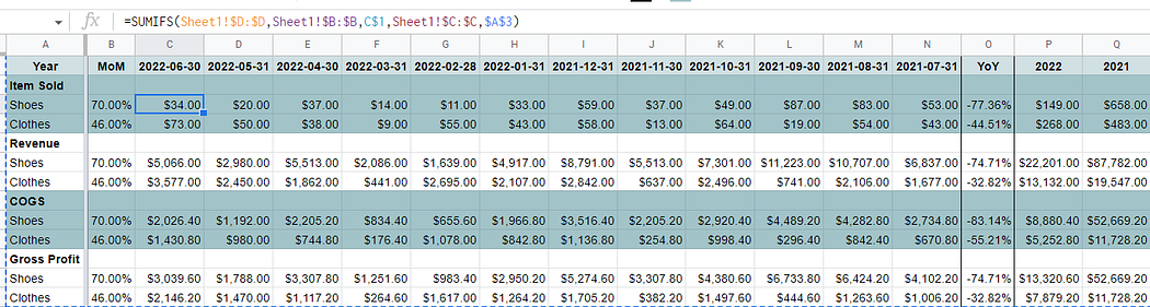
Example of SUMIFS function by Author

Finally, we can add the Month-on-Month and Year-on-Year simple calculations for trend analysis.

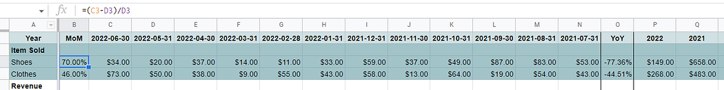
Example of month-on-month calculation by Author

BONUS: IMPORTRANGE

This particular function is very useful if you need to get raw data from another sheet, external or multiple Google Sheet sources becuase it imports the whole column and is precisely the same as the source column, hence no update is needed.

To illustrate, the Date and Item Name columns are imported from the raw sheet to the Copy of raw sheet. Always remember to add “ ” otherwise the formula won’t work.

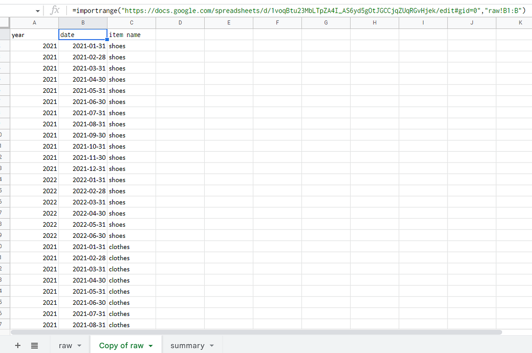
Example of Importrange function by Author

Manually changing and updating reports can be really tiring and mundane work :(. Therefore, let’s try to effectively reduce waste and automate it instead.